High dimensional data reduction and visualization with an example: digit recognition

Introduction

Dimensional reduction is the transformation of high-dimensional data into a low dimension representation. During this process, some information is lost but the main features are (hopefully!) preserved.

The elephant in the room of Machine Learning…

These transformations are very important because processing and analyzing high-dimensional data can be intractable. Dimension reduction is thus very useful in dealing with large numbers of observations and variables and is widely used in many fields.

Here we’ll approach three different techniques:

1. Principal component analysis (PCA)
2. Multidimensional Scaling (MDS)
3. Stochastic Neighbor Embedding (SNE)

PCA tries to project the original high-dimensional data into lower dimensions by capturing the most prominent variance in the data.

MDS is a technique for reducing data dimensions while attempting to preserve the relative distance between high-dimensional data points.

SNE is a non-linear technique to “cluster” data points by trying to keep similar data points close to each other.

PCA and classical MDS share similar computations: they both use the spectral decomposition of symmetric matrices, but on different input matrices.

Principal component Analysis (PCA)

PCA is often used to find low dimensional representations of data that maximizes the spread (variance) of the projected data.

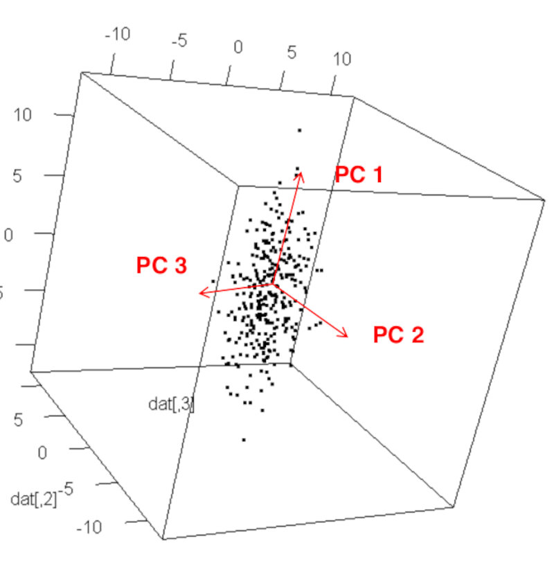
• The first principal component (PC1) is the direction of the largest variance of the data.
• The second principal component (PC2) is perpendicular to the first principal component and is the direction of the largest variance of the data among all directions that are perpendicular to the first principal component.
• The third principal component (PC3) is perpendicular to both first and second principal components and is in the direction of the largest variance among all directions that are perpendicular to both the first and second principal components.

This can continue until we obtain as many principal components as the dimensions of the original space in which the data is given, i.e. an orthogonal basis of the data space consisting of principal components.

Principal component analysis can be formulated in the following three equivalent ways. For simplicity, we will only formulate the problem for the first principal component.

Let $x^{(1)},x^{(2)},…,x^{(n)} \in \mathbb{R}^p$ denote $n$ data points in $p$ dimensional space. Without loss of generality, we assume that the data is centered at the origin (i.e. $\sum_{i=1}^n x^{(i)} = 0$). The first PC is the line spanned by a unit vector $w \in \mathbb{R}^p$ such that

• $\mathbf{w}$ minimizes the sum of squared residuals of the orthogonal projections of data $x^{(i)}$ onto $w$,

• $\mathbf{w}$ maximizes the sum of squared norms of the orthogonal projections of data $x^{(i)}$ onto $w$,

• $\mathbf{w}$ is an eigenvector corresponding to the largest eigenvalue of the sample covariance matrix $\mathbf{S}$,

To find the second principal component, we can repeat the process on the data projected into the space that is orthogonal to PC1, and so on.

Note: by definition, PCA gives linear projections into lower dimensional subspaces.

Note: PCA applies even when to data without any labels.

We can decide how many PCs to retain in the projection of the data based on their explained variance.

The total variance is the sum of variance of all the PCs, which equals to the sum of the eigenvalues of the covariance matrix,

The fraction of variance explained by a PC is the ratio of the variance of that PC to the total variance.

Multidimensional Scaling (MDS)

Multidimensional scaling (MDS) is a non-linear dimensionality reduction method to extract a lower-dimensional configuration from the measurement of pairwise distances (dissimilarities) between the points in a dataset.

Classical MDS

Let $x^{(1)},x^{(2)},…,x^{(n)} \in \mathbb{R}^p$ denote $n$ data points in $p$ dimensional space, and let the distance matrix $\mathbf{D} \in \mathbb{R}^{n\times n}$ consists of the elements of distances between each pair of the points, i.e. $d_{i,j} = \left| {x^{(i)}-x^{(j)}}\right|$.

The objective of MDS is to find points $y^{(1)},…,y^{(n)}\in\mathbb{R}^q$ in a lower dimensional space ($q < p$), such that the sum of all pairwise distances

is minimized.

The resulting points $y^{(1)},…,y^{(n)}$ are called a lower-dimensional embedding of the original data points.

Weighted MDS

Besides the above classical MDS, there are variations of MDS that use different objective functions.

The weighted MDS uses the objective function

where $w_{ij} \ge 0$ is the assigned weight.

Non-metric MDS

The non-metric MDS uses the objective function

in which we also optimize the objective over an increasing function $\theta$.

Note: non-classical MDS the objective functions are non-convex!

Stochastic Neighbor Embedding (SNE)

Stochastic neighbor embedding (SNE) is a probabilistic approach to dimensional reduction that places data points in high dimensional space into low dimensional space while preserving the identity of neighbors. That is, SNE attempts to keep nearby data points nearby, and separated data points relatively far apart.

The idea of SNE is to define a probability distribution on pairs of data points in each of the original high dimensional space and the target low dimensional space, and then determine the placement of objects in low dimension by minimizing the “difference’ of the two probability distributions.

So we’ll have

1. An input. The distance matrix $D_{ij}$ of the data in a p-dimensional space.

2. In the high dimensional $p$ space, center a Gaussian distribution on each data point $\mathbf{x}^{(i)}$, and define the probability of another data point $\mathbf{x}^{(j)}$ to be its neighbor to be

where the denominator sums over all distinct pairs of data points. Notice the symmetry $p_{ij} = p_{ji}$. Hence we can restrict to indices where $i < j$, and the above definition turns to

The shape of the Gaussian distribution ensures that pairs that are close together are given much more weight than pairs that are far apart.

1. In the low dimensional target space do the same procedure as in the previous point: define for each point $y^{(i)}$ the probability of $y^{(j)}$ being its neighbor to be

The set of all $q_{i,j}$ define the pmf of a probability distribution Q on all pairs of points in the q-dimensional target space.

1. Minimization. Find the points $\mathbf{y}^{(i)}$ in the q-dimensional target space than minimize the Kullback-Leibler (KL) divergence between the probability distributions P and Q,

where $p_{ij}$ and $q_{ij}$ vie the pmfs of P and Q respectively. In practice this minimization is implemented using gradient descent methods.

Note: these definitions are simplified, using the same variance at each datapoint.

T-SNE

One popular variation of SNE is the t-distributed stochastic neighbor embedding, which uses the t-distribution instead of the Gaussian distribution to define the pdf of neighbors in the low-dimensional target space. This means that

The heavy tail of the t-distribution reduces the problem of data points crowding in the middle.

Dimension reduction example: digit recognition

In this example we will use data from a demo from the python package scikit-learn: manifold learning on handwritten digits.

Loading the digits dataset

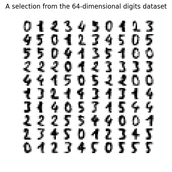
First we load the digits and use only 6 digits (0 to 5) for clarity. The digits look like the ones shown in the following picture.

#Adapted from:
#https://scikit-learn.org/stable/auto_examples/manifold/plot_lle_digits.html
# Authors: Fabian Pedregosa 
#          Olivier Grisel 
#          Mathieu Blondel 
#          Gael Varoquaux
#          Guillaume Lemaitre
# License: BSD 3 clause (C) INRIA 2011

from sklearn.datasets import load_digits
import matplotlib.pyplot as plt
import numpy as np

digits = load_digits(n_class=6)
X, y = digits.data, digits.target #X is the handwritten image, y is the number for training
n_samples, n_features = X.shape
n_neighbors = 30

We can plot the first 100 hand-written digits to show what we’re up against.

fig, axs = plt.subplots(nrows=10, ncols=10, figsize=(6, 6))
for idx, ax in enumerate(axs.ravel()):
    ax.imshow(X[idx].reshape((8, 8)), cmap=plt.cm.binary)
    ax.axis("off")
fig.suptitle("A selection from the 64-dimensional digits dataset", fontsize=16)

Note: 64 dimensions means we have 8x8 pixel images with 14 shades of gray (plus black and white).

Adding a function to plot the embedding

The function below will plot the projection of the original data onto each embedding and help us visualize the quality of the clustering and its variance.

rom matplotlib import offsetbox

from sklearn.preprocessing import MinMaxScaler


def plot_embedding(X, title):
    _, ax = plt.subplots()
    X = MinMaxScaler().fit_transform(X)

    for digit in digits.target_names:
        ax.scatter(
            *X[y == digit].T,
            marker=f"${digit}$",
            s=60,
            color=plt.cm.Dark2(digit),
            alpha=0.425,
            zorder=2,
        )
    shown_images = np.array([[1.0, 1.0]])  # just something big
    for i in range(X.shape[0]):
        # plot every digit on the embedding
        # show an annotation box for a group of digits
        dist = np.sum((X[i] - shown_images) ** 2, 1)
        if np.min(dist) < 4e-3:
            # don't show points that are too close
            continue
        shown_images = np.concatenate([shown_images, [X[i]]], axis=0)
        imagebox = offsetbox.AnnotationBbox(
            offsetbox.OffsetImage(digits.images[i], cmap=plt.cm.gray_r), X[i]
        )
        imagebox.set(zorder=1)
        ax.add_artist(imagebox)

    ax.set_title(title)
    ax.axis("off")

Embedding techniques comparison

Below, we compare different techniques. However, there are a couple of things to note:

• We will compare 13 techniques, from which we only discussed two: MDS and T-SNE. AS we’ll observe, they’re one of the most adequate to tackle this particular problem.
• We must note however, that each method has parameters that need to be fine-tuned (take a look at each method’s page at scikit-learn.org), and each method has its strong points and limitations: a method that does not work in one context may be the best in other. That is why is is best to test with many methods as possible, if you start with very little information.

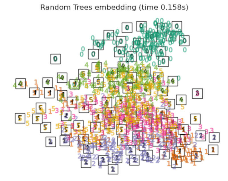
• the RandomTreesEmbedding is not technically a manifold embedding method, as it learn a high-dimensional representation on which we apply a dimensionality reduction method. However, it is often useful to cast a dataset into a representation in which the classes are linearly-separable.

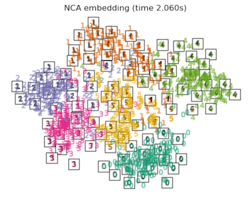
• the LinearDiscriminantAnalysis and the NeighborhoodComponentsAnalysis, are supervised dimensionality reduction method, i.e. they make use of the provided labels, contrary to other methods.

• the TSNE is initialized with the embedding that is generated by PCA in this example. It ensures global stability of the embedding, i.e., the embedding does not depend on random initialization.

# import methods
from sklearn.decomposition import TruncatedSVD
from sklearn.discriminant_analysis import LinearDiscriminantAnalysis
from sklearn.ensemble import RandomTreesEmbedding
from sklearn.manifold import (
    MDS,
    TSNE,
    Isomap,
    LocallyLinearEmbedding,
    SpectralEmbedding,
)
from sklearn.neighbors import NeighborhoodComponentsAnalysis
from sklearn.pipeline import make_pipeline
from sklearn.random_projection import SparseRandomProjection

embeddings = {
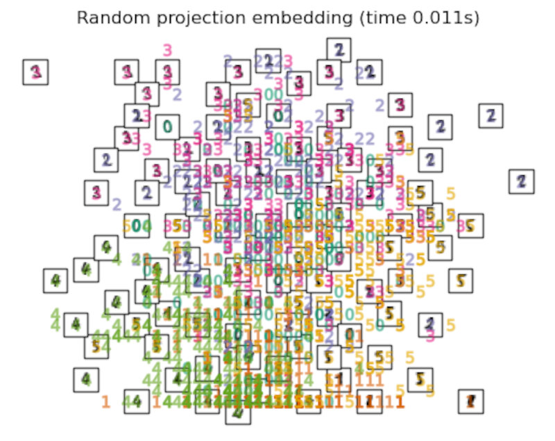
    "Random projection embedding": SparseRandomProjection(
        n_components=2, random_state=42
    ),
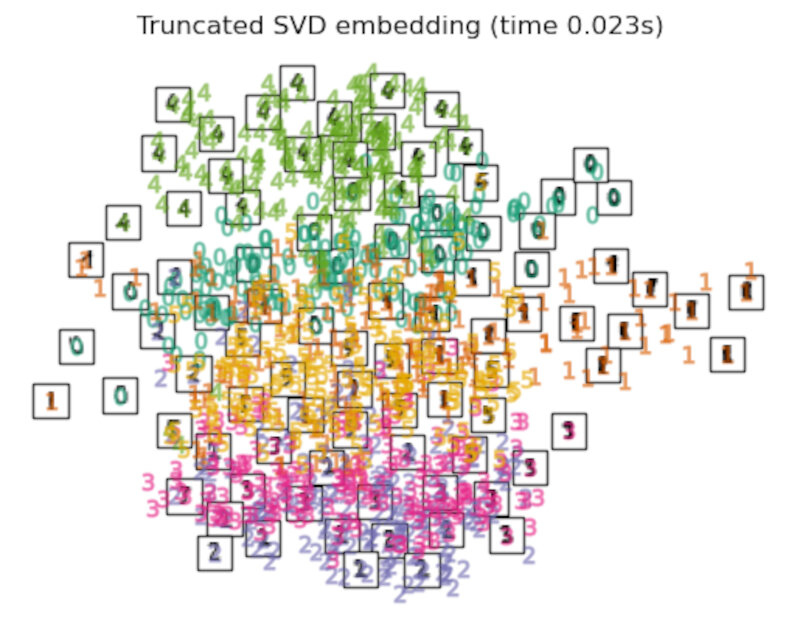
    "Truncated SVD embedding": TruncatedSVD(n_components=2),
    "Linear Discriminant Analysis embedding": LinearDiscriminantAnalysis(
        n_components=2
    ),
    "Isomap embedding": Isomap(n_neighbors=n_neighbors, n_components=2),
    "Standard LLE embedding": LocallyLinearEmbedding(
        n_neighbors=n_neighbors, n_components=2, method="standard"
    ),
    "Modified LLE embedding": LocallyLinearEmbedding(
        n_neighbors=n_neighbors, n_components=2, method="modified"
    ),
    "Hessian LLE embedding": LocallyLinearEmbedding(
        n_neighbors=n_neighbors, n_components=2, method="hessian"
    ),
    "LTSA LLE embedding": LocallyLinearEmbedding(
        n_neighbors=n_neighbors, n_components=2, method="ltsa"
    ),
    "MDS embedding": MDS(
        n_components=2, n_init=1, max_iter=120, n_jobs=2, normalized_stress="auto"
    ),
    "Random Trees embedding": make_pipeline(
        RandomTreesEmbedding(n_estimators=200, max_depth=5, random_state=0),
        TruncatedSVD(n_components=2),
    ),
    "Spectral embedding": SpectralEmbedding(
        n_components=2, random_state=0, eigen_solver="arpack"
    ),
    "t-SNE embeedding": TSNE(
        n_components=2,
        n_iter=500,
        n_iter_without_progress=150,
        n_jobs=2,
        random_state=0,
    ),
    "NCA embedding": NeighborhoodComponentsAnalysis(
        n_components=2, init="pca", random_state=0
    ),
}

Once we declared all the methods of interest, we can run and perform the projection of the original data. We will store the projected data as well as the computational time needed to perform each projection.

from time import time

projections, timing = {}, {}
for name, transformer in embeddings.items():
    if name.startswith("Linear Discriminant Analysis"):
        data = X.copy()
        data.flat[:: X.shape[1] + 1] += 0.01  # Make X invertible
    else:
        data = X

    print(f"Computing {name}...")
    start_time = time()
    projections[name] = transformer.fit_transform(data, y)
    timing[name] = time() - start_time

Computing Random projection embedding...
Computing Truncated SVD embedding...
Computing Linear Discriminant Analysis embedding...
Computing Isomap embedding...
Computing Standard LLE embedding...
Computing Modified LLE embedding...
Computing Hessian LLE embedding...
Computing LTSA LLE embedding...
Computing MDS embedding...
Computing Random Trees embedding...
Computing Spectral embedding...
Computing t-SNE embeedding...
Computing NCA embedding...

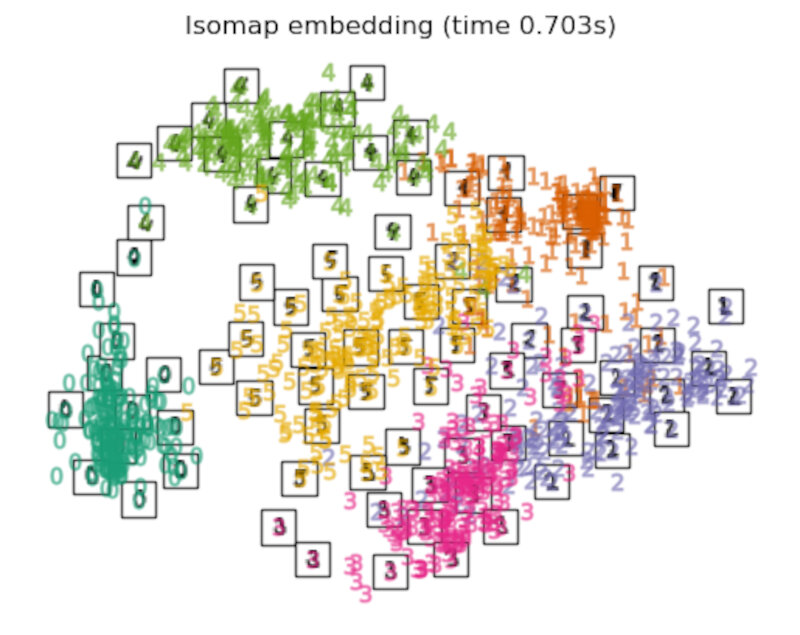
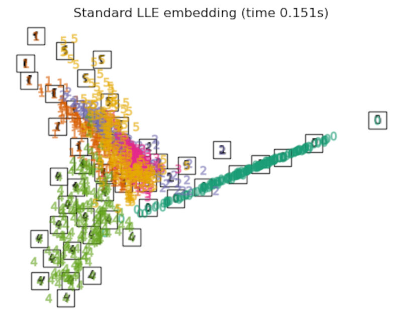
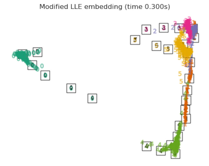
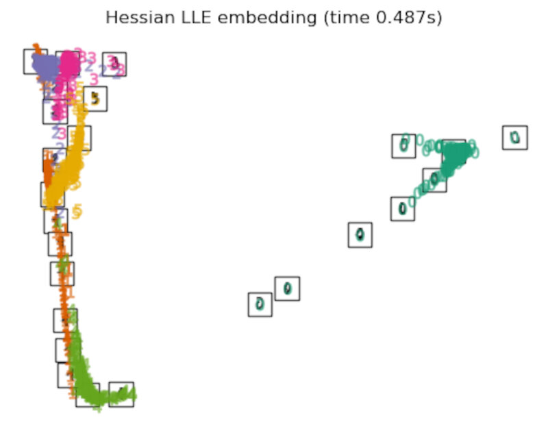
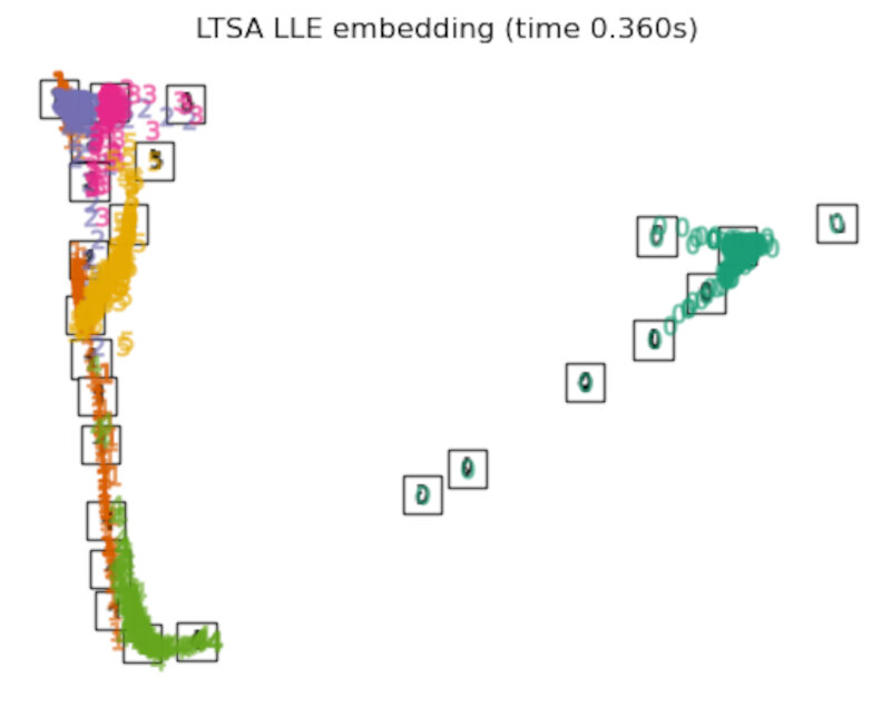
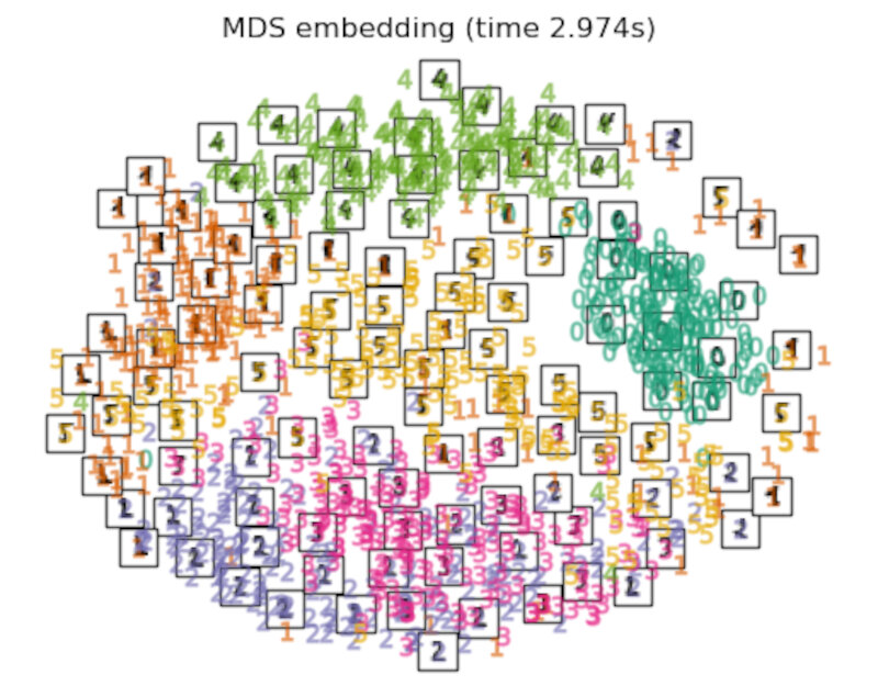
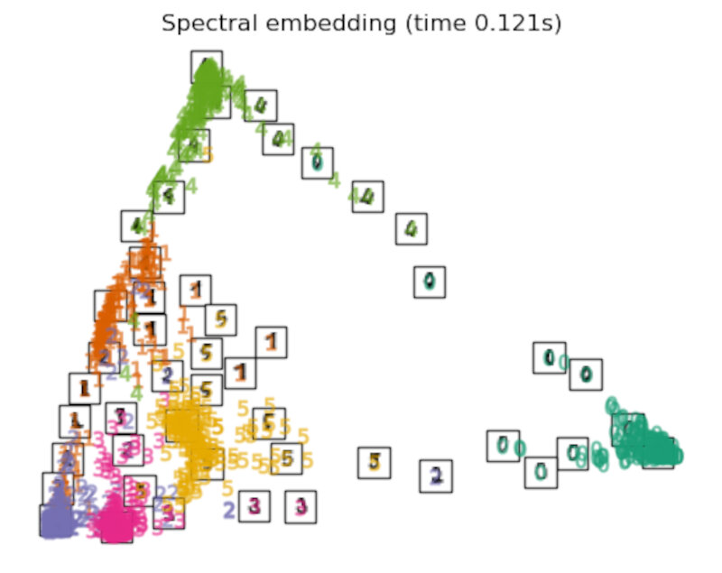
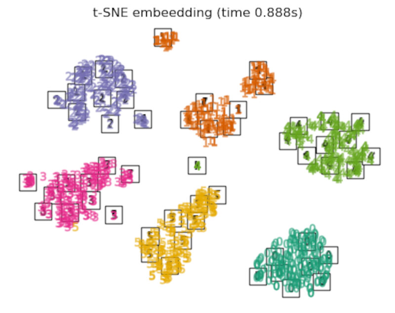
Finally, we can plot the resulting projection given by each method.

for name in timing:
    title = f"{name} (time {timing[name]:.3f}s)"
    plot_embedding(projections[name], title)

plt.show()

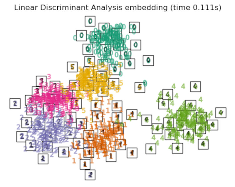
Discussion

• After performing a quick comparison we can conclude that the best technique for this specific problem is the t-sne: the cluster are clearly separated, ensuring a very high accuracy. MDS on the other hand shows some scattering but is still somewhat acceptable. It all depends on the level of error we are willing to tolerate.

• We could now establish some rules based, for instance, on the distance to the center of each cluster, to be able to read more hand-written numbers correctly.

• We should also be aware of the time each algorithm spends looking for the best solution. In this case, it is clear that the fastest algorithms do not work well, which, in any case, does not imply that the slowest ones are the best. The final choice depends on the problem at hand and on our computational resources.
• These approaches should be compared against deep learning methods (e.g. CNNs). This comparison may be a subject for a future post.