Resume

In this post I will present two different types of clinical trials: a discrete variable example and a continuous variable example showcasing a few different approaches on how to tackle these kinds of problems. It is also a good opportunity to present some fundamental statistical concepts. Towards the end we will revisit the Mammography study using this time the likelihood ratio approach and the last section will highlight the importance of doing p-value corrections when dealing with multiple hypothesis.

Mammography study - a discrete variable example

Here I will demonstrate how we can analyze data from observational studies using a mammography study as an example.

The key questions here are the following:

• Does mammography speeds up cancer detection?

• How do we set up an experiment in order to minimize the problem of confounding?

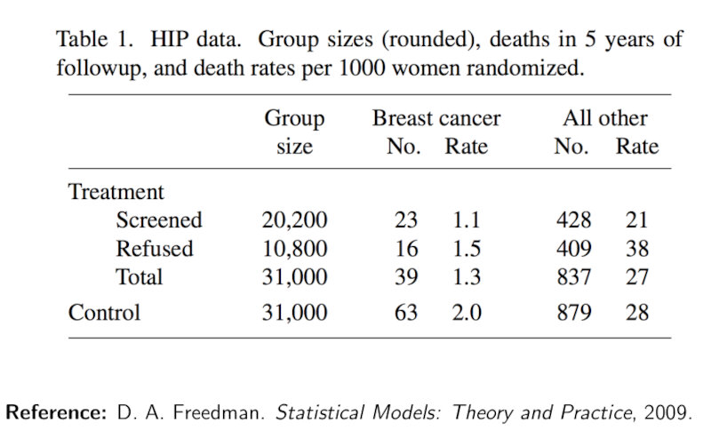
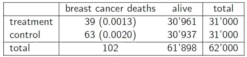
The study consists in the screening of women’s breasts by X-rays as shown in the Table below.

Intuitively, we are inclined to compare between those who took the treatment with the ones how refused it. However this is an observational comparison!

Instead we need to compare the whole treatment group against the whole control group.

We need to do an intent-to-treat analysis.

From the table we will assume that the outcome variable will be death by breast cancer. This variable will depend on the treatment variable, that will be the people offered mammography.

Why? Because we cannot force people to do the mammography!

RCT

In this experimental design we need to consider the following properties:

• Patient selection: Some populations are more likely to develop breast cancer than others depending on their prior health background, so the interpretation of any result we obtain will depend on how we have defined our selection procedure. In general, how we select the treatment and control groups will influence the population for which the conclusion is valid.

• Control group: We need to compare the outcome variable for those who have received the treatment with a baseline (i.e, the control group). Here, the control group (who were not offered a mammography) must be a comparable set of people to the treatment group (who have been offered a mammography).

• Features of the patients: One way to make accurate comparison and interpretation of results is to ensure that the treatment group is representative across factors such as health status, age, and ethnicity, and is similar along these dimensions as the control group. This way, we can attribute any differences in outcome to the treatment rather than differences in covariates. In a general study, it is upon the researchers’ discretion to determine which features to be careful about.

An experimental design where treatments are assigned at random and that satisfies the three points described above is called a randomized controlled trial (RCT). The controls can be an observational group or treated with a placebo.

Double blind

In any experiment that involves human subjects, factors related to human behavior may influence the outcome, obscuring treatment effects. For example, if patients in a drug trial are made aware that they actually received the new treatment pill, their behavior may change in a number of ways, such as by being more or less careful with their health-related choices. Such changes are very difficult to model, so we seek to minimize their effect as much as possible.

The standard way to resolve this is through a double-blind study, also called a blinded experiment. Here, human subjects are prevented from knowing whether they are in the treatment or control groups. At the same time, whoever is in charge of the experiment and anyone else who could interact with the patient are also prevented from directly knowing whether a patient is in the treatment or the control group. This is to prevent a variety of cognitive biases such as observer bias or confirmation bias that could influence the experiment.

In some cases, it is impossible to ensure that a study is completely double-blind. In the mammography study, for example, patients will definitely know whether they received a mammography. If we modify the treatment instead to whether a patient is offered mammography (which they could decline), then we neither have nor want double-blindness.

Hypothesis testing

From the table we can observe that

• death rate from breast cancer in control group = $\frac{63}{31k}$ = 0.0020
• death rate from breast cancer in treatment group = $\frac{39}{31k}$ = 0.0013

Key question: Is the difference in death rates between treatment and control sufficient to establish that mammography reduces the risk of death from breast cancer?

We need to perform an hypothesis test.

Hypothesis testing steps:

1. Determine a model. In our case Binomial (modeling as the outcome of a number n of heads/tails) or a Poisson model (modeling as number of arrivals/events).

2. Determine a mutually exclusive null hypothesis and alternative.

• $H_0$: $\pi = 0.002$ or $\lambda = 63$

• $H_1$: $\pi = 0.0013$ or $\lambda = 39$

1. Determine a test statistic (quantity that can differentiate between $H_0$ and $H_1$ and whose assumptions under $H_0$ are true)

T = #Deaths under $H_0$:

• T ~ Binomial(31k,0.002)

or

• T ~Poisson(63)

1. Determine a significance level ($\alpha$) i.e. the probability of rejecting $H_0$ when $H_0$ is true: e.g. $\alpha \le 0.05$.

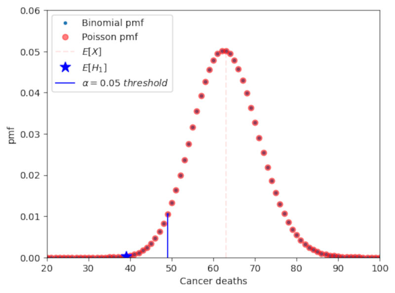
The following Figure shows the pmf of a Binomial and a Poissonian distributions. The significance level is depicted as the dashed blue line. We can observe that the distributions are very similar. Therefore, for large n, it is preferred to use the Poissonian approximation.

In this case, if the p-value of the test statistic is lower than 0.05 we can say that we reject the null at the 0.05 confidence level. In practice, however, we should be very careful about the importance of p-values and should use other statistical tools as well as we’ll see later on.

Code:

import numpy as np
from scipy.stats import poisson,binom
import matplotlib.pyplot as plt

n = 31000 #control sample size
death = 63 # number of cancer deaths in control
rate = death/n #death ratio in control
x = np.arange(0,125) #parameter space
#binomial calculation exercise
pmf_binomial = binom.pmf(x,n,rate)

#poisson approximation
pmf_poisson = poisson.pmf(x,death)

alpha = x[np.where(np.cumsum(pmf_binomial) <= 0.05)][-1] #alpha = 0.05

plt.plot(x,pmf_poisson,'.',label='Binomial pmf')
plt.plot(x,pmf_poisson,'or',alpha=0.5,label='Poisson pmf')
plt.plot((63,63),(0,0.05),'r--',alpha=0.1,label='$E[H_0]$')
plt.plot(39,pmf_binomial[39],'b*',markersize=12,label='$E[H_1]$')
plt.plot((alpha,alpha),(0,pmf_binomial[alpha]),'b-',label="$\\alpha=0.05\ threshold$")
plt.xlabel('Cancer deaths'),plt.ylabel('pmf')
plt.xlim(20,100),plt.ylim(0,0.06)

plt.legend()

The p-value is calculated by summing all pmf values up to pmf(x=39). Therefore, the p-value is a probability. In this case we obtain a value of 0.0008 which is much smaller than 0.05. Thus, we reject the null.

We can now define type I error, type II error and power from the following table.

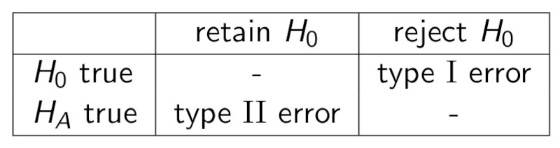
Type I error is a false positive and is bounded by $\alpha$ (meaning type I error $\le \alpha$), Type II error is a false negative, and the power can be written as

Note: there is a trade-off between type I error and type II error.

Note: the power of a 1-sided test is usually higher than the power of a 2-sided test. Thus you should always use 1-sided tests when evaluating deviations that go in one direction only.

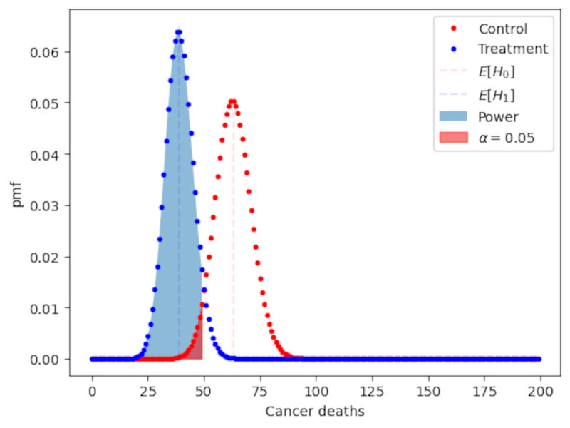
The following plot shows a graphical depiction of the power of the test as well as the upper bound of the Type I error represented by $\alpha$. The plot clearly shows the interplay between type I and type II errors:

Fisher exact test

What if we don’t know the frequency of deaths of the control? We can do a Fisher exact test which is based on the hypergeometric distribution.

Null hypothesis: $\pi$ control = $\pi$ treatment

Alternative hypothesis: $\pi$ control > $\pi$ treatment

Key question: Knowing that 102 subjects died and that number of treatments / controls each is 31k what is the probability that deaths are so unevenly distributed?

The $\textit{p-value}$ is then the sum of probabilities of obtaining a value of T that is more extreme than 39, in the direction of the alternate hypothesis:

$\textit{p-value} = 0.011 < 0.05$

From here, based on the significance level $\alpha$, we can either

• reject the null if $p \le \alpha$

or

• fail to reject the null if $p > \alpha$.

Advantages:

• Does not assume knowledge about the true probability of dying due to breast cancer in the control population

Shortcomings:

• Assumes knowledge of the margins (i.e., row and column sums)
• Alternative is Bernard’s test (estimates the margins)
• Both tests are difficult to perform on large tables for computational reasons

Sleeping drug study - a continuous variable example

Let’s now move on to a different study where we have a continuous variable as our variable of interest.

In the clinical trial setup we are testing a new sleeping aid drug which in principle should help users suffering from insomnia to increase their sleeping time.

Which should be the best approach to this problem?

We could adapt the previous framework for the mammography study. However, the power of this hypothesis might not be very high, considering that the sample size is small: people have a wide range of sleep lengths and may be difficult to discern anything due to this natural variability. An alternative to the standard RTC test is a paired test design.

Paired test design

In the paired test design one takes multiple samples from the same individual at different times, a group corresponding to the control situation and the other group corresponding to the treatment situation. This allow us to estimate the effect of the drug at the individual level.

Therefore we will measure the difference between the observed values in the treatment and in the control situations,

The null hypothesis is the one where the expected value of the measurement $E[Y_i] = 0$.

Note: the paired test design removes the need for randomization. However the individual does not know if he is in the treatment or the in the control group. This can be done by having two seperate observation periods: one for a placebo administration and the other for the drug treatment.

Modeling choice for the sleeping drug study

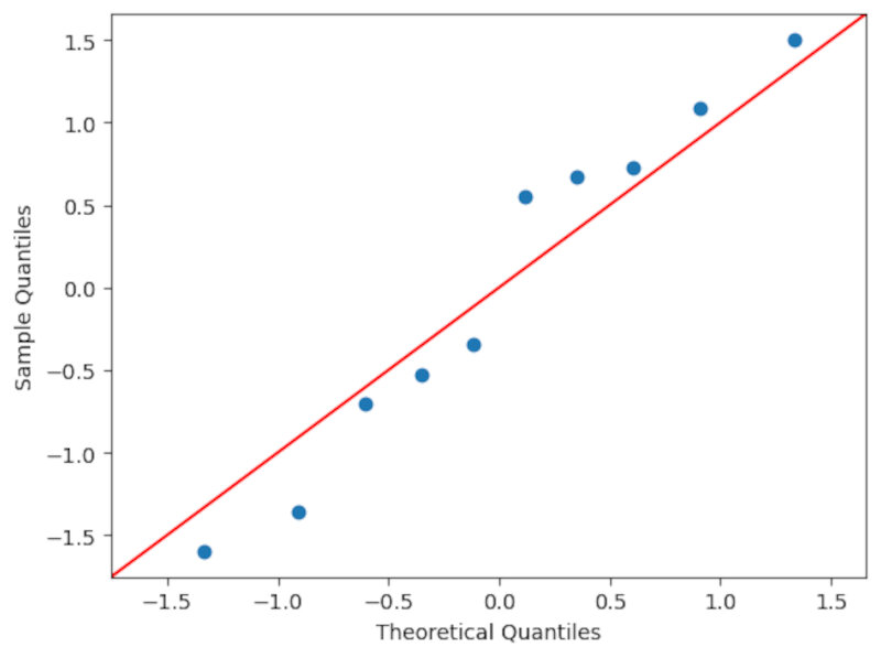
The following table shows the data collected for our clinical trial.

What should be our modeling choice?

In this case we can think in two possibilities a priori:

• The number of hour slept in a day has an upper bound, as shown in the table which implies that the difference $Y$ is also bounded. This points in favour of the uniform distribution as this model has bounded support, while the Gaussian distribution has infinite support.

• We can look at the empirical distribution of the observations. The number of hours slept by an adult is known to be centered around 8 hours, and outliers are rare, so this favours the Gaussian distribution model.

In this case, it is preferable to choose the Gaussian distribution as it closely matches the empirical distribution of the sleeping population. We can further argue that the number of hours slept is a cumulative effect of a large number of biological and lifestyle variables. As most of these variables are unrelated to each other, the cumulative effect can be approximated by a normal distribution.

The central limit theorem (CLT) and the z-test statistic

From the CLT, we know that when $n$ is large, the distribution of the random variables of a sample $X_1…X_n$ is approximately normal with mean $\mu$ and variance $\sigma^2$. Therefore,

From here we can define a test statistic, the z-test statistic as

This test statistic does not depend on the parameters $\mu$ or $\sigma$. It is, in fact, the standard normal. Thus we can simply use the CDF of this function to calculate the $\textit{p-value}$ of the test statistic.

In our case we want to answer the following question:

Does the drug increase hours of sleep enough to matter?

To answer this question we go through the following steps:

1. Choose a model (Gaussian) and use the proper random variables ($Y_i = X_{drug}-X_{placebo}$).
2. State the hypothesis (in this case is a one-sided test):
   • $H_0$: $\mu = 0$.
   • $H_1$: $\mu > 0$.
3. Calculate the test statistic.

We have, however, a problem. To calculate z we need to known the true value of the variance $\sigma$. Since we do not know the population variance, only the sample variance we cannot use this test.

T-test

The solution to this problem is to use a t-test instead. The t-test uses the sample variance, and enable us to write

under the assumption that $X_1,…,X_n \sim N(\mu,\sigma)$. This distribution is called a t-distribution and is parameterized by a number of degrees of freedom. In this case, $T \sim t_{n-1}$, the t distribution with $n-1$ degrees of freedom, where $n$ is the number of samples.

Application to the sleeping drug experiment

To calculate the T-test to our experiment we first calculate the difference of the hours of sleep between drug and placebo as shown in the table below.

Then, we know that under the null the t-test follows a t distribution of 9 degrees of freedom,

Using for instance the t-test program in the scipy python library we obtain

t_test = sp.stats.ttest_1samp(x,0,alternative='greater') #note: alternative='greater' because by default the t-test output is a two-sided test.
print ('The t-test statistic =',t_test[0], 'with a p-value =',t_test[1],'and df = 9.')
The t-test statistic = 3.1835383022188735 with a p-value = 0.005560692749284678 and df = 9.

In this case we can also reject the null at the 5% level (or even at the 1% level).

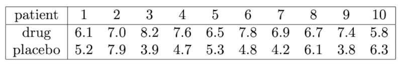
The pdf of a $t_9$ distribution is shown below and compared to a standard normal distribution.

Code:

df = 9 #number of degrees of freedom
x = np.linspace(-5,5,1000) #support
td = sp.stats.t.pdf(x,df)
tn = sp.stats.norm.pdf(x)

indx = np.max(np.where(x<t_test[0])) #location of the pdf value of the t-score

plt.plot(x,td,'r',label='T-distribution (df=9)')
plt.plot(x,tn,'b',label='Z distribution')
plt.plot(t_test[0],td[indx],'*k',label='T score',markersize=12)

plt.legend()

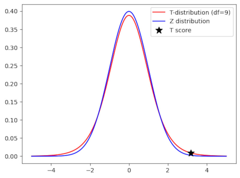
A great feature of the $t_n$ distribution is that it introduces uncertainty due to the estimation of the population variance: As $n$ gets smaller and smaller the tails of the T distribution get larger and larger as shon in the following Figure.

Note: as a rule of thumb, when the sample size $n \ge 30$ the t-distribution is already very similar to the normal distribution. At this threshold the normal approximation becomes (more) valid.

Other basic statistical concepts

Testing the assumption of normality

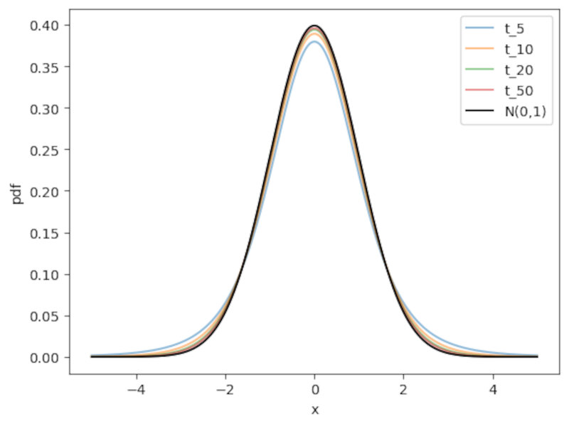
• When using a t-test sometimes we have very few samples. It is thus important to check the assumption of normality of the random variables. How can we do that?

  • Using a qq-plot (quantile-quantile plot). By inspecting the form of the qq plot one has a qualitative measure of the form of the distribution. In this example I use the qqplot function of the statsmodels library. In short the function draws at random $n$ numbers and orders them, doing the same with the sample values. Then, if they’re more or less in a straight line we can have some confidence that our sample is drawn from a normal distribution. It’s important to note that it is necessary to subtract by the mean and divide by the standard deviation to properly use the qq plot.
  • Using a KS test (one sample Kolmogorov smirnov test of normality). For instance we can use the 1-sample KS test for normality contained in the scipy.stats library and we conclude that there is a high probability that our data is drawn from a normal distribution ($\textit{p-value} \sim 0.64$) as shown below. Always take care to check if you’re doing a 1-sided or a two-sided test.

Code:

sp.stats.ks_1samp(teste,sp.stats.norm.cdf,alternative='greater')
KstestResult(statistic=0.13524505784239993, pvalue=0.6393148695381738, statistic_location=-0.34577756840579527, statistic_sign=1)

The Wilcoxon signed-rank test

Ok, but what if the assumption of normality is not valid? What if the sample has origin in any other distribution?

You can use the Wilcoxon sign-rank test. You just need to ensure that the sample are drawn from some distribution that is symmetric around a mean.

• Model: $X_1…X_n \sim Dist. $ symmetric around a mean $\mu$.
• Test statistic: $W=\sum{_{i=1}^n X_i-\mu}R_i$, where $R_i$ is the rank of $| X_i-\mu|$. The rank is just a weight that gives a value of 1 to the smallest distance and a value of $n$ to the largest distance.
• This test statistic is asymptotically normal.

There are many other tests. The most important thing is to always check the assumption of each test very carefully!

Confidence intervals

Ok, we’re now actually happy with our model to obtain the expected value and its variability. But actually we’re more interested in a range of realistic values. How should we quantify this range?

This range is called a confidence interval. It is centered around the sample mean and its width is proportional to the standard error.

The interval is defined in such a way that with probability $1-\alpha$ the interval will contain the true mean $\mu$. In other words, if we sample the dataset many times and calculate intervals each time, the probability that $\mu$ is in the proposed range is $1-\alpha$.

We can write this interval in the following way

where $\phi$ is the cdf of the distribution and $\alpha$ is the significance level.

If we isolate $\mu$ then we obtain

Therefore, the (two-sided in this case!) confidence interval will be

To better understand what the confidence interval is we can create a very simple simulation where we randomly draw 100 elements from a standard normal distribution 100 times. The result is depicted in the following Picture.

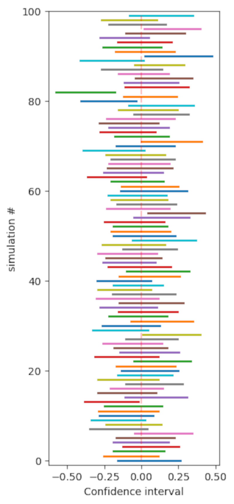
Here we assume that $\alpha = 0.05$ and thus $\Phi^{-1}_{0.975} \sim 1.96$.

Code:

#simulation
#100 sets of 100 standard gaussian distribution draws
#here we assume alpha = 0.05
#we know the table value of phi^-1(0.95) = P(z<1.96) = 1.96
q = 1.96 #alpha quantile for alpha=0.05
media = np.zeros(100)
ci = np.zeros((100))
plt.figure(figsize=(3,8))
for n in range(100) :
    dist = sp.stats.norm.rvs(size=100)
    media[n] = dist.mean()
    ci[n] = dist.std()/np.sqrt(len(dist))*q
    plt.plot((media[n]-ci[n],media[n]+ci[n]),(n,n),linewidth=2)

plt.plot((media.mean(),media.mean()),(0,99),'r--',alpha=0.25,label='$\mu$')
plt.xlabel('Confidence interval'),plt.ylabel('simulation #')
plt.ylim(-1,100)

A general approach: the likelihood ratio test

The likelihood ratio test is quite important because

• you can use it in any setting
• is quite powerfull! From the Neyman-Pearson Lemma, the likelihood raio test is the most powerful among all $\alpha$ tests for testing $H_0: \theta=\theta_0$ versus $H_A: \theta = \theta_A$ so it should be used in these cases.

In general terms we can write that

• We can have a model with r.v. X $\sim$ Distribution(x,$\theta$), where $\theta$ are the paremeters
• We want to do a test on a null hypothesis $H_0: \theta \in \Theta_0 $ versus $H_A: \theta \in \Theta_A$, where $\Theta_0 \cap \Theta_A = \emptyset$
• The likelihood ratio will be $L(X) = \frac{\max_{\theta \in \Theta_0 p(x;\theta)}}{\max_{\theta \in \Theta p(x;\theta)}}$, where $\Theta = \Theta_0 \cup \Theta_A$. Also,
  • $0 \le L(x) \le 1$
  • if $L(x) « 1, \theta \in \Theta_A$
  • if $L(x) \sim 1, \theta \in \Theta_0$
  • the numerator is the maximum of the probability of observing the data under the null.
  • the denominator is the maximum of the probability that you observe the data that you are given.
  • the parameter $\theta$ that maximizes $p(x;\theta)$ is called the maximum likelihood estimator (MLE).
  • the parameter $\theta$ can be in the null model or in the alternative model!
• The likelihood raio test
  • will reject $H_0$ if $L(x) < \eta$, where $\eta$ is chosen such that $P_H0(L(x) \le \eta) = \alpha$

Looks very complicated! How do we calculate this thing?

In general $L(x)$ does not have an easily computable null distribution. To actually compute it, we need to do the following transformation

where

• $0 \le \Lambda(x) \le \inf$
• reject $H_0$ if $\Lambda(x)$ is too large.
• From the Wilks Theorem we know that, under H_0

where $d = dim(\Theta) - dim(\Theta_0) >0$.

Still looks very cryptic…

Let’s go back to the HIP mammography cancer study. The table below shows our data.

In this case we have

• $H_0: \pi_{treatment} = \pi_{control}$ versus $H_A: \pi_{treatment} \ne \pi_{control}$
• We’re in the binomial framework. Therefore we need to calculate the binomial distribution probabilities for each case. Let $Y_T$ and $Y_C$ be the numbers of cancer deaths in the treatment and control groups respectively. Assumming that these groups are independent from each other, the probability of having y_t cancer deaths in the treatment group and y_c deaths in the control group is

$Y_T$ and $Y_C$ will be

and

Ok, let’s calculate the LR test step-by-step!

The initial equation is

The maximum values of the probabilities are obtained with MLE estimators, so we can write that

• Under $H_0$ the MLE is $\hat{\pi}$ and

• Under $H_A$ the MLEs are $\hat{\pi}{treatment}$ and $\hat{\pi}{control.}$, and

To calculate the MLE estimators we need to transform the probability into a logarithm and then derive to find the maximum. Doing the two simple operations we end up with (surprise!):

• $\hat{\pi} = \frac{102}{62k}$
• $\hat{\pi}_{treat} = \frac{39}{31k}$
• $\hat{\pi}_{control} = \frac{63}{31k}$

Now, we just need to plug-in the values into the formula above and we get

Computing the test in python just takes one line of code.

LRtest = -2*np.log(sp.stats.binom.pmf(39,31000,102/62000)*sp.stats.binom.pmf(63,31000,102/62000)/(sp.stats.binom.pmf(39,31000,39/31000)*sp.stats.binom.pmf(63,31000,63/31000)))
print ('The value of the LR test is',LRtest)
The value of the LR test is 5.709660479762173

Under the null, the Wilks theorem states that this distribution tends to a $\chi$ squared distribution of degree $d$, where $d = 2-1$.

Therefore, we will observe where the value of the test ended up in this distribution as shown below.

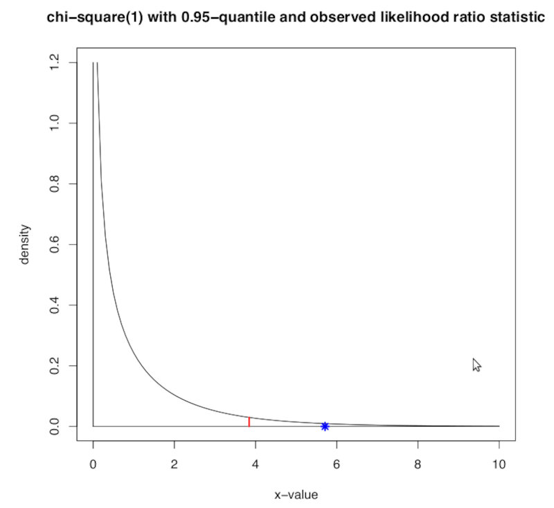
The $\alpha$ threshold is depicted by the red line and our test value is shwon as the blue star. As we can clearly see, according to the likelihood ratio test, for a significance value $\alpha = 0.05$ we can safely reject $H_0$.

We can also calculate the $\textit{p-value}$. In this case it will be the probability above the test value. We can obtain this value using the cdf of this function.

The cdf will give the probability up to $x=5.71$. To obtain the p-value we just obtain the remaining part of the probability by calculating the complement $1-cdf$. Again we just need one line of code.

pvalue = 1-sp.stats.chi2.cdf(5.71,1)
print('The p-value associated to the LR test is',pvalue)
The p-value associated to the LR test is 0.016868539397458027

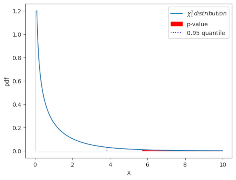
We can also observe this p-value graphically as shown in the following plot.

Code:

x = np.linspace(0.1,10,1000)
pdf_x = sp.stats.chi2.pdf(x,1)
q_alfa = 3.84 #0.95 quantile taken from table
f_alfa = pdf_x[np.max(np.where(x<=q_alfa))]

plt.plot(x,pdf_x,label='$\chi^2_1 distribution$')
plt.fill_between(x,pdf_x,color='red',where=(x>=LRtest),label='p-value')
plt.plot((q_alfa,q_alfa),(0,f_alfa),'b:',label='0.95 quantile')
plt.plot((0,0),(0,1.2),'k',linewidth=0.5)
plt.plot((0,10),(0,0),'k',linewidth=0.5)
plt.xlabel('X'),plt.ylabel('pdf')

plt.legend()

Multiple hypothesis testing

So far we’ve seen cases for single hypothesis testing, but in the real world and in a lot of experiments there are at least a few variables that need to be taken into account.

There is also the temptation that, when doing an experiment, to test for as many variables as possible. This has the awful side effect of increasing the chances of finding spurious correlations.

For instance:

• Intake of tomato sauce (p-value of 0.001), tomatoes (p-value of 0.03), and pizza (p-value of 0.05) reduce the risk of prostate cancer;
• But for example tomato juice (p-value of 0.67), or cooked spinach (p-value of 0.51), and many other vegetables are not significant.
• ”Orange cars are less likely to have serious damages that are discovered only after the purchase.”

See where we are going?

For instance consider the case of a famous product called “Wonder-syrup”. To study the benefits of ingesting this syrup, a research group constructed the following experiment:

• they choose a randomized group of 1000 people.
• measured 100 variables before and after taking the syrup: weight, blood pressure, etc.
• performed a paired t-test with a significance level of 5\%.

If we model the number of false significant tests as having a Binomial distribution, or Binom(100,0.05), on average we will get 5 out of 100 variables showing a significant effect!!

*How can we prevent this from happening in multiple hypothesis testing?

We need to correct our p-values!

There are two main avenues to consider:

• Family-wise error rate (FWER) which is the probability of making at least one false discovery, or type I error.

and

• False discovery rate (FDR) which is the expected fraction of false significance results among all significance results.

Family-wise error rate (FWER)

FWER is usually used when we really need to be careful and control the error rate dut to possible serious consequences in any false discovery, such as the Pharmaceutical sector.

We can control the size of the FWER by choosing significance levels of the individual tests to vary with the size of the series of tests. This translates to correcting the p-values before comparing with a fixed significance level e.g. $\alpha = 0.05$.

Bonferroni Correction

The simples of the possible correction for $\alpha$ is the Bonferroni Correction. If we have $m$ tests performed at the same time, the corrected p-value will be

then $FWER < \alpha$. We can re-write the equation stating that

Note: We should note that this is a very stringent and conservative test, and can be applied when the tests are not necessarily independent of each other. Note: when $m$ is large this criteria are stringent and lowers the power of the tests.

Holm-Bonferroni Correction

The Holm-Bonferroni method is more flexible and less stringent.

Suppose we have $m$ hypothesis. The application of the method consists in the following steps:

• Calculate the initial p-values for each hypothesis.
• Sort the initial p-values in increasing order.
• Start with the p-value with the lowest number. If

then

• reject $H_0^i$
• proceed to the next smallest p-value by 1, and again use the same rejection criterion above.
• As soon as hypothesis $H_0^k$ is not rejected, stop and do not reject any more of the $H_0$.

Note: This procedure guarantees $FWER < \alpha$ for $m$ tests, which do not need to be independent. Note: the Holms-Bonferroni method is more powerful than the Bonferroni correction, since it increases the chance of rejecting the null hypothesis, and thus reduces the change of type II errors.

False discovery rate (FDR)

In most cases, however, FWER is too strict and we loose too much statistical power. The most sensible course of action is then to control the expected proportion of false discoveries among all discoveries made. We can define

The Benjamini-Hochberg correction

The Benjamini-Hochbert correction guarantees $FDR < \alpha$ for a series of $m$ independent tests..

The method is as follows:

• Sort the $m$ p-values in increasing order.
• Find the maximum $k$ such that

• Reject all of $H_0^1, H_0^2,…,H_0^k.$

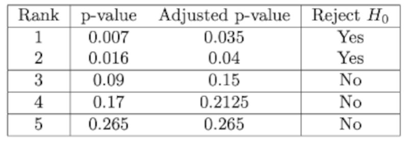
Example

The table below illustrates how to apply the method. First we rank the p-values, then we calculate the adjusted value and then we reject the ones with $p<\alpha$.

Commonly accepted practice

What correction should we use and in which settings?

• It’s ok not correcting for multiple testing when generating the original hypothesis, but the number of tests performed must be reported. Generally, to check
• If it’s a screening or exploratory analysis you do want to get some significant results. Then, a $FDR \le 10\%$ is adequate.
• In more stringent contexts like confirmatory analysis you really need to use a $FWER \le 5\%$, like for instance the test done by the Food and Drug Administration.
• Personally, and in general, I would go for a FDR between 1 to 5% but it all depends on the context, type of sample, sample number, variables, error type, etc.